Intro Stata
Introduction to Stata
Link to YouTube Video Lecture
Click the image below:
Materials and setup
Laptop users: you will need a copy of Stata installed on your machine.
- You can install a licensed version from https://warwick.ac.uk/services/its/servicessupport/software/list/stata
- Find class materials at Click to Download
- Download and extract to your desktop or any folder of your choice!
Section descripton
- This is an introduction to Stata
- Assumes no/very little knowledge of Stata
- Not appropriate for people already well familiar with Stata
- Learning Objectives:
- Familiarize yourself with the Stata interface
- Get data in and out of Stata
- Compute statistics and construct graphical displays
- Compute new variables and transformations
Why stata?
- Used in a variety of disciplines
- User-friendly
- Great guides available on web
- Freely available - Warwick Staff & Students
Stata interface
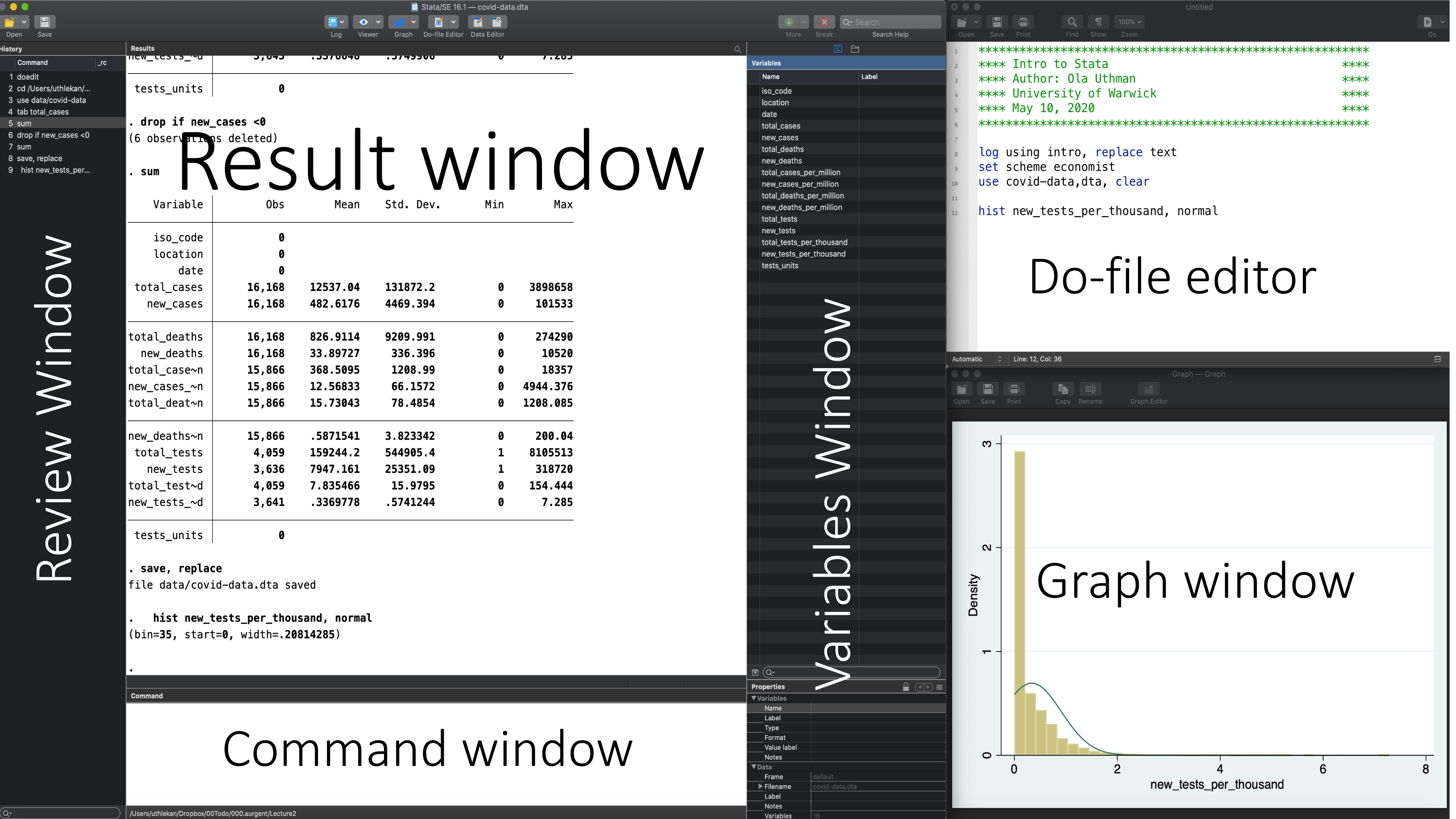
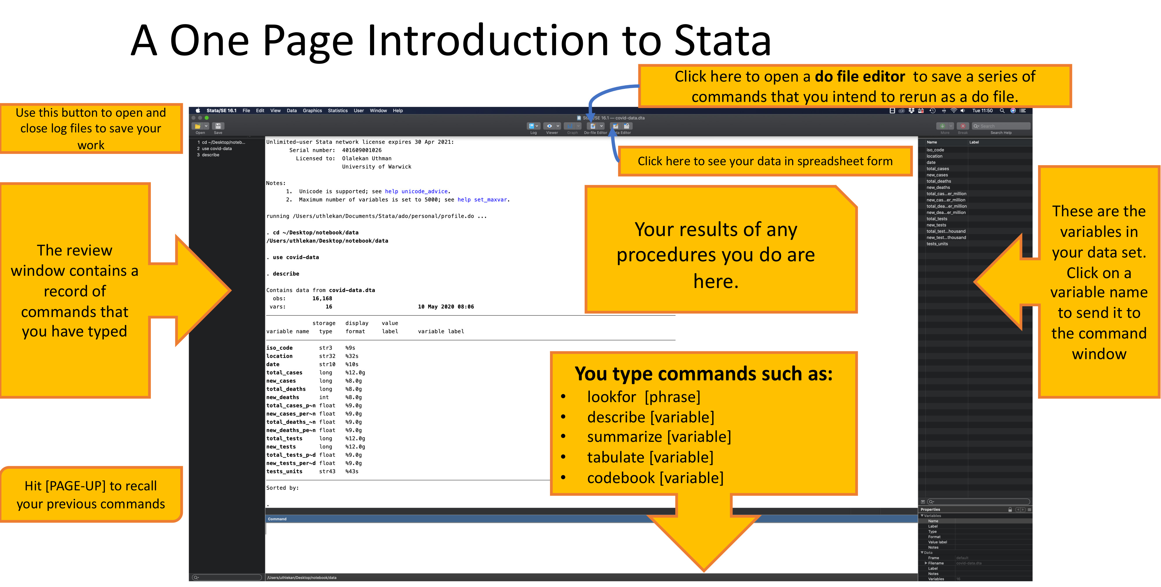
Do-files
- You can type all the same commands into the Do-file that you would type into the command window
- BUT…the Do-file allows you to save your commands
- Your Do-file should contain ALL commands you executed – at least all the “correct” commands!
- I recommend never using the command window or menus to make CHANGES to data
- Saving commands in Do-file allows you to keep a written record of everything you have done to your data
- Allows easy replication
- Allows you to go back and re-run commands, analyses and make modifications
Stata help
To get help in Stata type help followed by topic or command, e.g., help meta.
General Stata command syntax
Most Stata commands follow the same basic syntax: Command varlist, options
Commenting and formatting syntax
Start with comment describing your Do-file and use comments throughout
-
Use ‘*’ to comment a line and ‘//’ for in-line comments
-
Make Stata say hello:
disp "Hello " "World!" // 'disp' is short for 'display' -
Use /// to break varlists over multiple lines:
disp "Hello" /// " World!"
Let’s get started
-
Launch the Stata program
- Open up a new Do-file
- Run our first Stata code
-
change directory
// cd "C://Users/Desktop/StataIntro"
Getting data into Stata
Data file commands
- Next, we want to open our data file
- Open/save data sets with “use” and “save”:
cd data/

// open the covid-data.dta data set
use covid-data.dta, clear

// save data file:
save new-covid-data.dta, replace // "replace" option means OK to overwrite existing file
file new-covid-data.dta saved
A note about path names
- If your path has no spaces in the name (that means all directories, folders, file names, etc. can have no spaces), you can write the path as is
- If there are spaces, you need to put your pathname in quotes
- Best to get in the habit of quoting paths
What if my data is not a Stata file?
-
import data from a .csv file
import delimited data/covid-data.csv, clear
-
Import data from Excel
import excel using data/covid-data.xlsx, clear firstrow
Statistics and graphs
Frequently used commands
- Commands for reviewing and inspecting data:
- describe // labels, storage type etc.
- sum // statistical summary (mean, sd, min/max etc.)
- codebook // storage type, unique values, labels
- list // print actuall values
- tab // (cross) tabulate variables
- browse // view the data in a spreadsheet-like window
- Examples
summarize // statistical summary
    Variable |        Obs        Mean    Std. Dev.       Min        Max
-------------+---------------------------------------------------------
    iso_code |          0
    location |          0
        date |          0
 total_cases |     16,168    12537.04    131872.2          0    3898658
   new_cases |     16,168    482.6176    4469.394          0     101533
-------------+---------------------------------------------------------
total_deaths |     16,168    826.9114    9209.991          0     274290
  new_deaths |     16,168    33.89727     336.396          0      10520
total_case~n |     15,866    368.5095     1208.99          0      18357
new_cases_~n |     15,866    12.56833     66.1572          0   4944.376
total_deat~n |     15,866    15.73043     78.4854          0   1208.085
-------------+---------------------------------------------------------
new_deaths~n |     15,866    .5871541    3.823342          0     200.04
 total_tests |      4,059    159244.2    544905.4          1    8105513
   new_tests |      3,636    7947.161    25351.09          1     318720
total_test~d |      4,059    7.835466     15.9795          0    154.444
new_tests_~d |      3,641    .3369778    .5741244          0      7.285
-------------+---------------------------------------------------------
 tests_units |          0
codebook total_cases location // information about how total_cases & location are coded
--------------------------------------------------------------------------------
total_cases                                                          (unlabeled)
--------------------------------------------------------------------------------

                  type:  numeric (long)

                 range:  [0,3898658]                  units:  1
         unique values:  3,998                    missing .:  0/16,168

                  mean:     12537
              std. dev:    131872

           percentiles:        10%       25%       50%       75%       90%
                                 0         2        51       717      6879

--------------------------------------------------------------------------------
location                                                             (unlabeled)
--------------------------------------------------------------------------------

                  type:  string (str32)

         unique values:  211                      missing "":  0/16,168

              examples:  "Colombia"
                         "Hungary"
                         "Mexico"
                         "Seychelles"

               warning:  variable has embedded blanks
tab location // numbers of location
                        location |      Freq.     Percent        Cum.
---------------------------------+-----------------------------------
                     Afghanistan |        121        0.75        0.75
                         Albania |         62        0.38        1.13
                         Algeria |        126        0.78        1.91
                         Andorra |         57        0.35        2.26
                          Angola |         49        0.30        2.57
                        Anguilla |         44        0.27        2.84
             Antigua and Barbuda |         51        0.32        3.15
                       Argentina |         64        0.40        3.55
                         Armenia |        122        0.75        4.30
                           Aruba |         48        0.30        4.60
                       Australia |        131        0.81        5.41
                         Austria |        131        0.81        6.22
                      Azerbaijan |        124        0.77        6.99
                         Bahamas |         53        0.33        7.32
                         Bahrain |        130        0.80        8.12
                      Bangladesh |         66        0.41        8.53
                        Barbados |         53        0.33        8.86
                         Belarus |        124        0.77        9.62
                         Belgium |        131        0.81       10.43
                          Belize |         47        0.29       10.72
                           Benin |         54        0.33       11.06
                         Bermuda |         51        0.32       11.37
                          Bhutan |         57        0.35       11.73
                         Bolivia |         58        0.36       12.09
 Bonaire Sint Eustatius and Saba |         38        0.24       12.32
          Bosnia and Herzegovina |         58        0.36       12.68
                        Botswana |         39        0.24       12.92
                          Brazil |        131        0.81       13.73
          British Virgin Islands |         44        0.27       14.00
                          Brunei |         60        0.37       14.37
                        Bulgaria |         61        0.38       14.75
                    Burkina Faso |         58        0.36       15.11
                         Burundi |         39        0.24       15.35
                        Cambodia |        122        0.75       16.11
                        Cameroon |         58        0.36       16.46
                          Canada |        131        0.81       17.27
                      Cape Verde |         50        0.31       17.58
                  Cayman Islands |         51        0.32       17.90
        Central African Republic |         55        0.34       18.24
                            Chad |         51        0.32       18.56
                           Chile |         66        0.41       18.96
                           China |        131        0.81       19.77
                        Colombia |         66        0.41       20.18
                         Comoros |          8        0.05       20.23
                           Congo |         55        0.34       20.57
                      Costa Rica |         63        0.39       20.96
                   Cote d'Ivoire |         57        0.35       21.31
                         Croatia |        131        0.81       22.12
                            Cuba |         56        0.35       22.47
                         Curacao |         47        0.29       22.76
                          Cyprus |         59        0.36       23.13
                  Czech Republic |        131        0.81       23.94
    Democratic Republic of Congo |         58        0.36       24.29
                         Denmark |        131        0.81       25.11
                        Djibouti |         52        0.32       25.43
                        Dominica |         48        0.30       25.72
              Dominican Republic |        122        0.75       26.48
                         Ecuador |        124        0.77       27.25
                           Egypt |        127        0.79       28.03
                     El Salvador |         52        0.32       28.35
               Equatorial Guinea |         56        0.35       28.70
                         Eritrea |         49        0.30       29.00
                         Estonia |        131        0.81       29.81
                        Ethiopia |         57        0.35       30.16
                  Faeroe Islands |         51        0.32       30.48
                Falkland Islands |         36        0.22       30.70
                            Fiji |         51        0.32       31.02
                         Finland |        131        0.81       31.83
                          France |        131        0.81       32.64
                French Polynesia |         52        0.32       32.96
                           Gabon |         57        0.35       33.31
                          Gambia |         53        0.33       33.64
                         Georgia |        128        0.79       34.43
                         Germany |        131        0.81       35.24
                           Ghana |         57        0.35       35.60
                       Gibraltar |         51        0.32       35.91
                          Greece |        130        0.80       36.71
                       Greenland |         51        0.32       37.03
                         Grenada |         48        0.30       37.33
                            Guam |         52        0.32       37.65
                       Guatemala |         56        0.35       37.99
                        Guernsey |         51        0.32       38.31
                          Guinea |         56        0.35       38.66
                   Guinea-Bissau |         44        0.27       38.93
                          Guyana |         56        0.35       39.28
                           Haiti |         51        0.32       39.59
                        Honduras |         57        0.35       39.94
                       Hong Kong |          5        0.03       39.97
                         Hungary |         67        0.41       40.39
                         Iceland |        131        0.81       41.20
                           India |        130        0.80       42.00
                       Indonesia |        124        0.77       42.77
                   International |         63        0.39       43.16
                            Iran |        131        0.81       43.97
                            Iraq |        129        0.80       44.77
                         Ireland |        129        0.80       45.57
                     Isle of Man |         50        0.31       45.87
--more--
Basic graphing commands
- Univariate distribution(s) using hist
/* Histograms */
hist new_tests_per_thousand
(bin=35, start=0, width=.20814285)
// histogram with normal curve; see 'help hist' for other options
  hist new_tests_per_thousand, normal
(bin=35, start=0, width=.20814285)
gladder new_tests_per_thousand
/* scatterplots */
   twoway (scatter new_cases new_deaths)
graph matrix new_cases new_deaths new_tests
Working on subsets
- It is often useful to select just those rows of your data where some condition holds–for example select only rows where sex is 1 (male)
- The following operators allow you to do this:
| Operator | Meaning |
|---|---|
| == | equal to |
| != | not equal to |
| > | greater than |
| >= | greater than or equal to |
| < | less than |
| <= | less than or equal to |
| & | and |
| | | or |
- Note the double equals signs for testing equality
Generating and replacing variables
- Create new variables using “gen”
// create a new variable named mc_inc
  //   equal to inc minus the mean of inc
gen small_cases = new_cases < 1000
tab small_cases
small_cases |      Freq.     Percent        Cum.
------------+-----------------------------------
          0 |        808        5.00        5.00
          1 |     15,360       95.00      100.00
------------+-----------------------------------
      Total |     16,168      100.00
// categorical variable

recode new_cases ///
 (min / 999 = 1 "Very small number cases") ///
 (1000/9999 = 2 "Small number of cases")  ///
 (10000 / max = 3 "Very high number of cases"),  ///
 gen(cases_cat)

tab cases_cat
(15205 differences between new_cases and cases_cat)


      RECODE of new_cases |      Freq.     Percent        Cum.
--------------------------+-----------------------------------
  Very small number cases |     15,360       95.00       95.00
    Small number of cases |        695        4.30       99.30
Very high number of cases |        113        0.70      100.00
--------------------------+-----------------------------------
                    Total |     16,168      100.00
Exercise 4: Manipulating variables
- Use the dataset, covid-data.dta
- Generate a new variable, high_deaths greater than 1000
- Generate a new “deaths_cate” variable that will take on a value of “1” if number of total deaths < 1000; 2 between 1000 and 9999 and 3 greater than 10000
Wrap-up
Stata cheat sheets
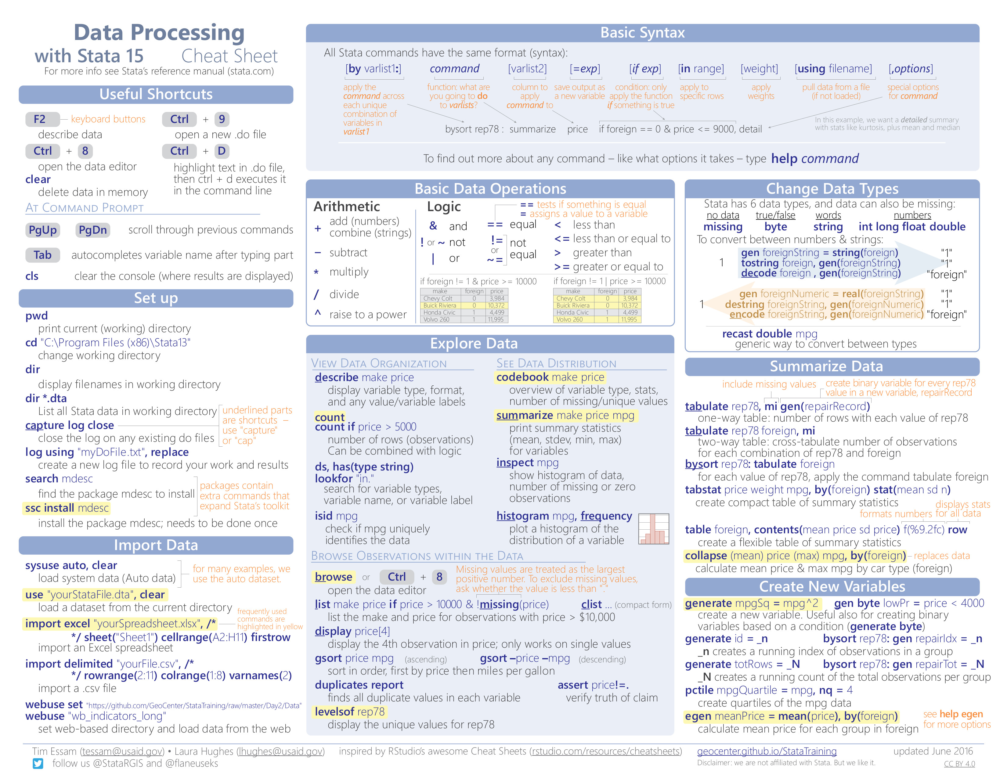
Basic Processing
- Fundamental commands in Stata to import, explore, summarize, and create new variables
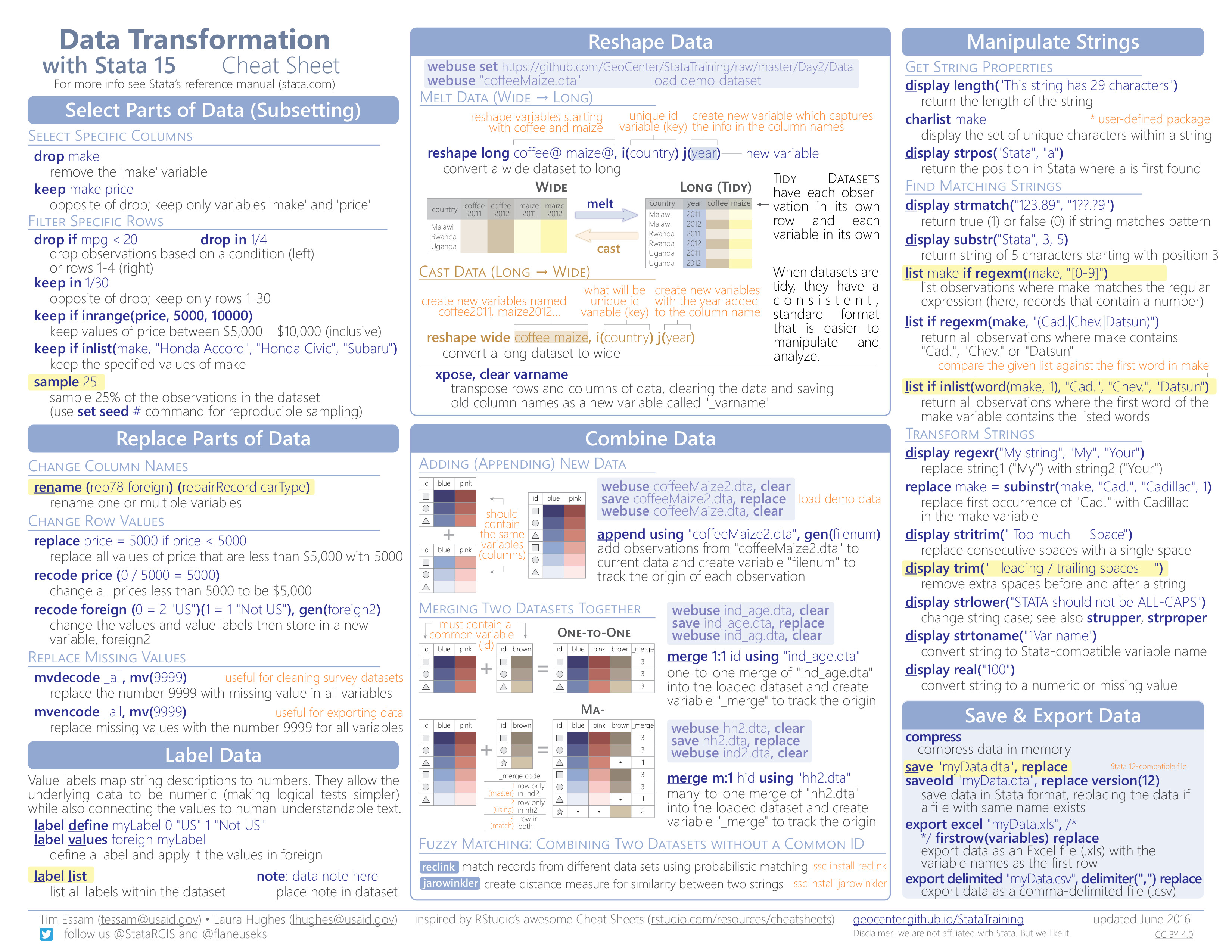
Data Transformation
- Selecting portions of datasets, replacing and labeling data, reshaping, merging, string manipulation, and saving
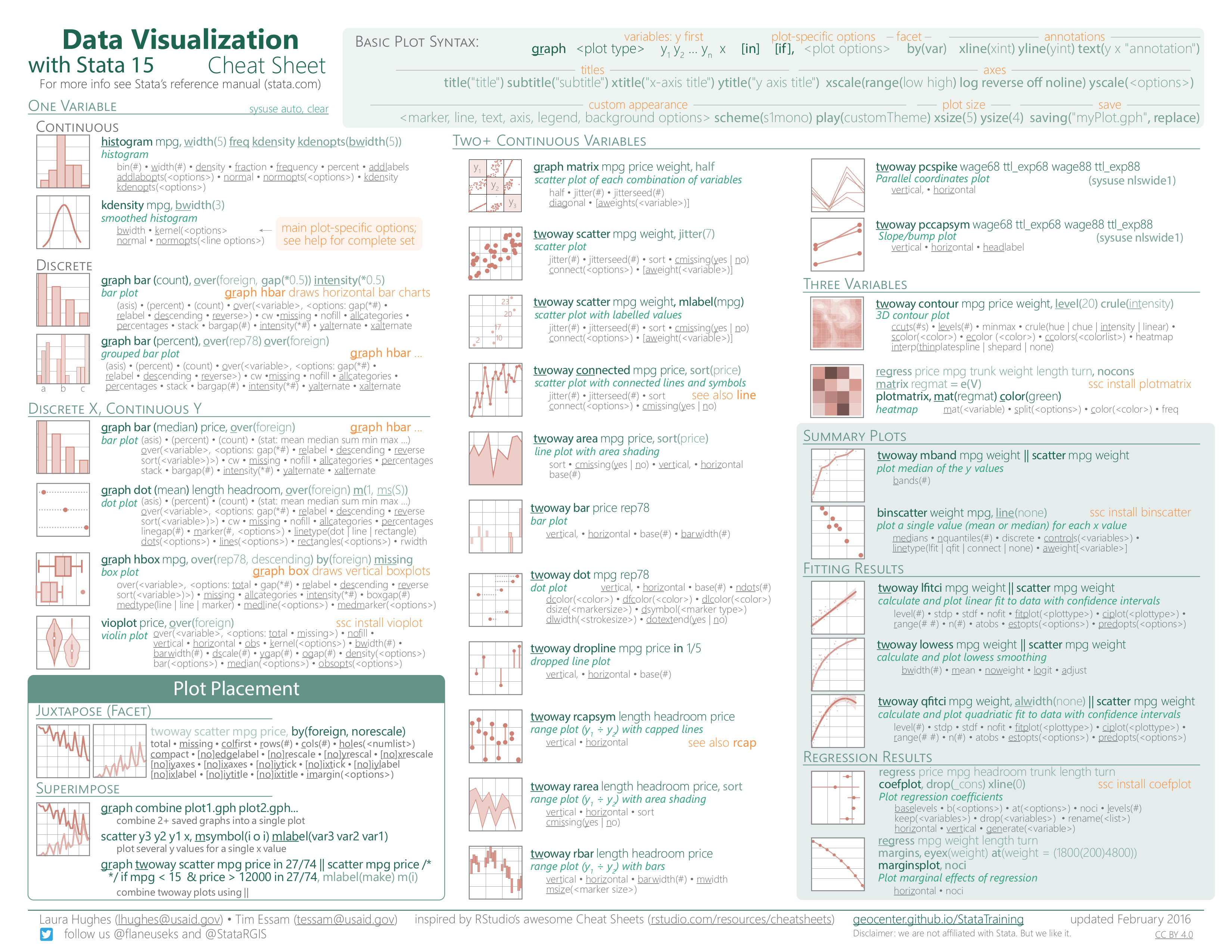
Creating Data Visualizations
- Syntax and arguments for plotting functions
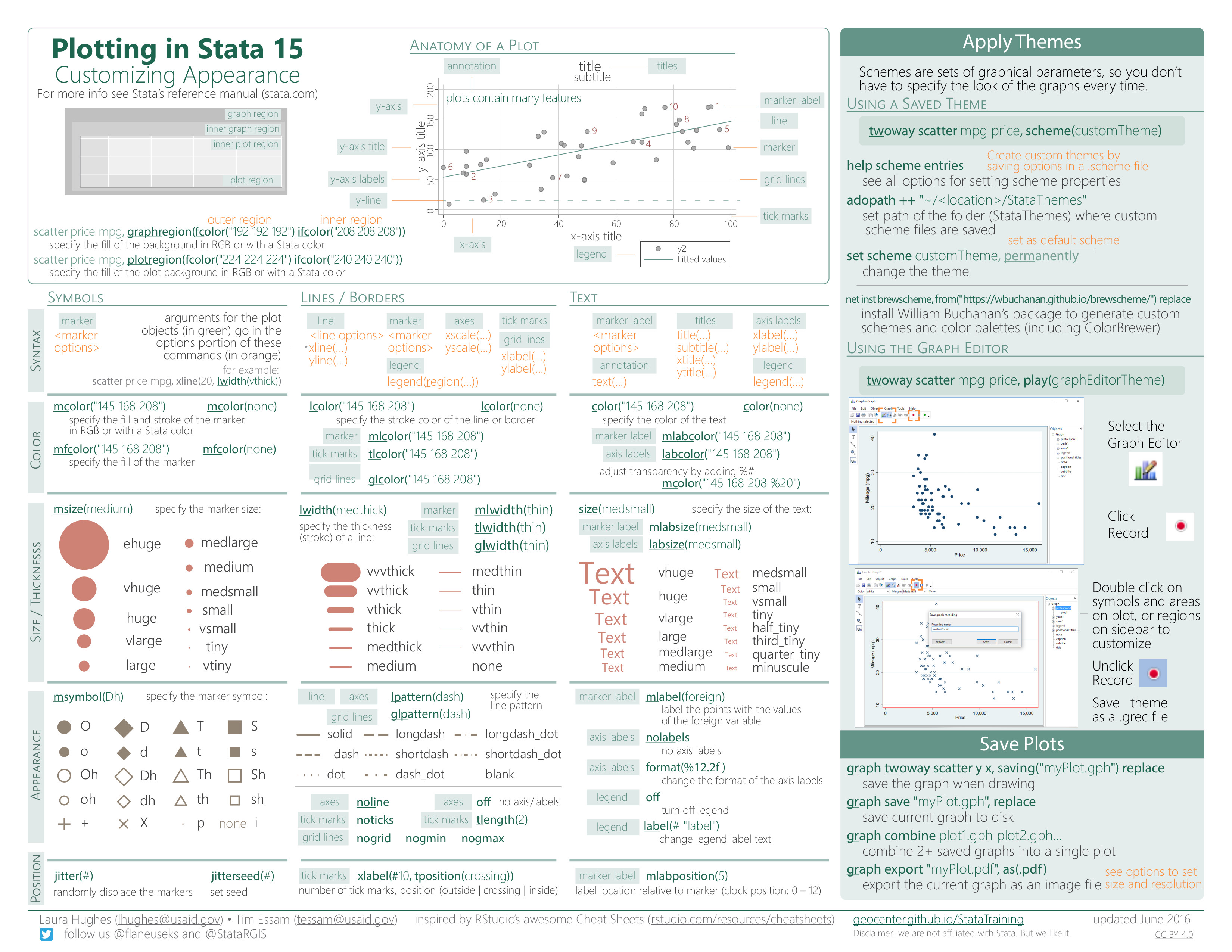
Customizing Data Visualizations
- Options to change the appearance of plots
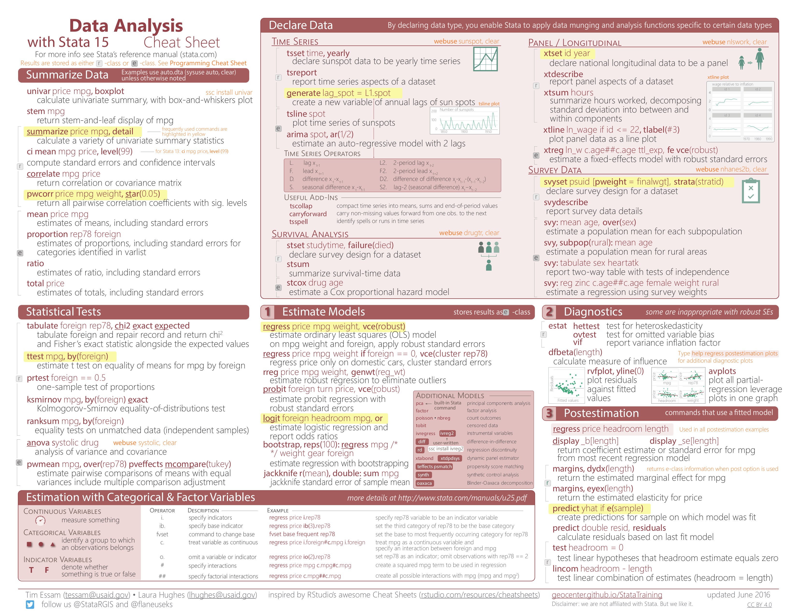
Data Analysis
- Summarize data, declare data, conduct statistical tests, and estimate models
